Classification using Transfer Learning(VGG16)

 

VGG16:

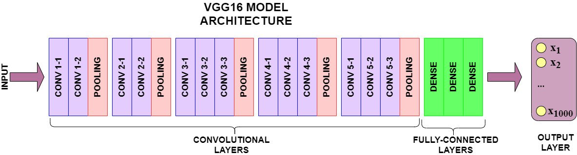
VGG16 is a convolutional neural network trained on a subset of the ImageNet dataset, a collection of over 14 million images belonging to 22,000 categories. K. Simonyan and A. Zisserman proposed this model in the 2015 paper, Very Deep Convolutional Networks for Large-Scale Image Recognition.

In the 2014 ImageNet Classification Challenge, VGG16 achieved a 92.7% classification accuracy. But more importantly, it has been trained on millions of images. Its pre-trained architecture can detect generic visual features present in our Food dataset.

Fig 2. The VGG16 Model has 16 Convolutional and Max Pooling layers, 3 Dense layers for the Fully-Connected layer, and an output layer of 1,000 nodes.

Now suppose we have many images of two kinds of cars: Ferrari sports cars and Audi passenger cars. We want to generate a model that can classify an image as one of the two classes. Writing our own CNN is not an option since we do not have a dataset sufficient in size. Here's where Transfer Learning comes to the rescue!

We know that the ImageNet dataset contains images of different vehicles (sports cars, pick-up trucks, minivans, etc.). We can import a model that has been pre-trained on the ImageNet dataset and use its pre-trained layers for feature extraction.

Now we can't use the entirety of the pre-trained model's architecture. The Fully-Connected layer generates 1,000 different output labels, whereas our Target Dataset has only two classes for prediction. So we'll import a pre-trained model like VGG16, but "cut off" the Fully-Connected layer - also called the "top" model.

Once the pre-trainedlayers have been imported, excluding the "top" of the model, we can take 1 of 2 Transfer Learning approaches.

1. Feature Extraction Approach

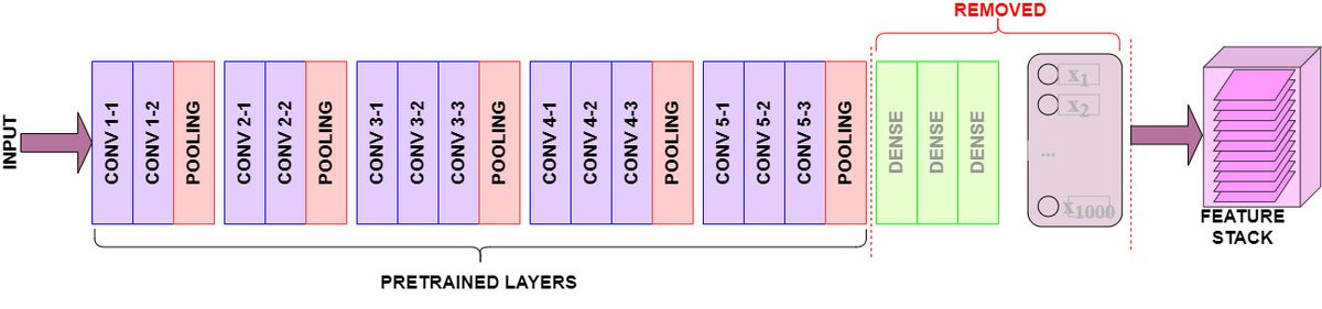
We use the pre-trained model's architecture to create a new dataset from our input images in this approach. We'll import the Convolutional and Pooling layers but leave out the "top portion" of the model (the Fully-Connected layer).

Recall that our example model, VGG16, has been trained on millions of images - including vehicle images. Its convolutional layers and trained weights can detect generic features such as edges, colors, wheels, windshields, etc.

We'll pass our images through VGG16's convolutional layers, which will output a Feature Stack of the detected visual features. From here, it's easy to flatten the 3-Dimensional feature stack into a NumPy array - ready for whatever modeling you'd prefer to conduct.

Fig 3. The above graphic shows the "top" portion of the model as removed. The model convolves the pre-trained output layers left behind as a 3D stack of feature maps.

We can do feature extraction in the following manner:

1. Download the pre-trained model. Ensure that the "top" portion of the model - the Fully-Connected layer - is not included.
2. Pass the image data through the pre-trained layers to extract convolved visual features
3. The outputted feature stack will be 3-Dimensional, and for it to be used for prediction by other machine learning classifiers, it will need to be flattened.
4. At this point, you have two options:
   1. Stand-Alone Extractor: In this scenario, you can use the pre-trained layers to extract image features once. The extracted features would then create a new dataset that doesn't require any image processing.
   2. Bootstrap Extractor: Write your own Fully-Connected layer, and integrate it with the pre-trained layers. In this sense, you are bootstrapping your own "top model" onto the pre-trained layers. Initialize this Fully-Connected layer with random weights, which will update via backpropagation during training.

This article will show how to implement a "bootstrapped" extraction of image data with the VGG16 CNN. Pre-trained layers will convolve the image data according to ImageNet weights. We will bootstrap a Fully-Connected layer to generate predictions.

2. Fine-Tuning Approach

In this approach, we employ a strategy called Fine-Tuning. The goal of fine-tuning is to allow a portion of the pre-trained layers to retrain.

In the previous approach, we used the pre-trained layers of VGG16 to extract features. We passed our image dataset through the convolutional layers and weights, outputting the transformed visual features. There was no actual training on these pre-trained layers.

Fine-tuning a Pre-trained Model entails:

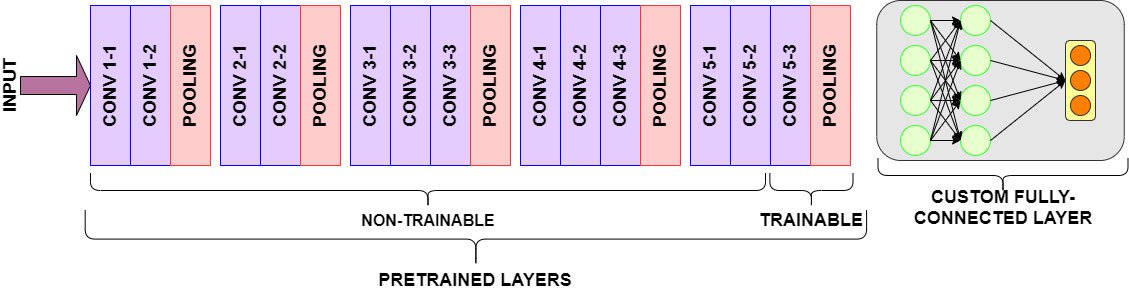
1. Bootstrapping a new "top" portion of the model (i.e., Fully-Connected and Output layers)
2. Freezing pre-trained convolutional layers
3. Un-freezing the last few pre-trained layers training.

The frozen pre-trained layers will convolve visual features as usual. The non-frozen (i.e., the 'trainable') pre-trained layers will be trained on our custom dataset and update according to the Fully-Connected layer's predictions.

Fig 4. In the above graphic representation, the final convolutional and pooling layers are unfrozen to allow training. A Fully-Connected layer is defined for training and prediction.

In this article, we will demonstrate how to implement Fine-tuning on the VGG16 CNN. We will load some of the pre-trained layers as 'trainable', pass image data through the pre-trained layers, and 'fine-tune' the trainable layers alongside our Fully-Connected layer.

Downloading the Dataset

Before we demonstrate either of these approaches, ensure you've downloaded the data for this tutorial.

To access the data used in this tutorial, check out the Image Classification with Keras article. You can find the terminal commands and functions for splitting the data in this section. If you're starting from scratch, make sure to run the split_dataset function after downloading the dataset so that the images are in the correct directories for this tutorial.

Using Transfer Learning for Food Classification

Pre-trained models, such as VGG16, are easily downloaded using the Keras API. We'll go ahead and use VGG16 for the tutorial, but you should explore the other models available! Many of them have been trained on the ImageNet dataset and come with their advantages and disadvantages. You can find a list of the available models here.

We've also imported something called a preprocess_function alongside the VGG16 model. Recall that image data must be normalized before training. Images are composed of 3-Dimensional matrices containing numerical values in a range of [0, 255]. Not all CNNs have the same normalization scheme, however.

The VGG16 model was trained on data wherein pixel values ranged from [0, 255], and the mean pixel values of the dataset are subtracted from each image channel.

Other models have different normalization schemes, details of which are in their documentation. Some models require scaling the numerical values to be between (-1, +1).

Preparing the training and testing data

Let's first import some necessary libraries.

import os
from keras.models import Model
from keras.optimizers import Adam
from keras.applications.vgg16 import VGG16, preprocess_input
from keras.preprocessing.image import ImageDataGenerator
from keras.callbacks import ModelCheckpoint, EarlyStopping
from keras.layers import Dense, Dropout, Flatten
from pathlib import Path
import numpy as np

In the previous article, we defined image generators (see here) for our particular use case. Now, we'll need to utilize the VGG16 preprocessing function on our image data.

BATCH_SIZE = 64

train_generator = ImageDataGenerator(rotation_range=90, 
                                     brightness_range=[0.1, 0.7],
                                     width_shift_range=0.5, 
                                     height_shift_range=0.5,
                                     horizontal_flip=True, 
                                     vertical_flip=True,
                                     validation_split=0.15,
                                     preprocessing_function=preprocess_input) # VGG16 preprocessing

test_generator = ImageDataGenerator(preprocessing_function=preprocess_input) # VGG16 preprocessing

With our ImageDataGenerator's, we can now flow_from_directory using the same image directory as the last article:

download_dir = Path('<your_directory_here>')

train_data_dir = download_dir/'food-101/train'
test_data_dir = download_dir/'food-101/test'

class_subset = sorted(os.listdir(download_dir/'food-101/images'))[:10] # Using only the first 10 classes

traingen = train_generator.flow_from_directory(train_data_dir,
                                               target_size=(224, 224),
                                               class_mode='categorical',
                                               classes=class_subset,
                                               subset='training',
                                               batch_size=BATCH_SIZE, 
                                               shuffle=True,
                                               seed=42)

validgen = train_generator.flow_from_directory(train_data_dir,
                                               target_size=(224, 224),
                                               class_mode='categorical',
                                               classes=class_subset,
                                               subset='validation',
                                               batch_size=BATCH_SIZE,
                                               shuffle=True,
                                               seed=42)

testgen = test_generator.flow_from_directory(test_data_dir,
                                             target_size=(224, 224),
                                             class_mode=None,
                                             classes=class_subset,
                                             batch_size=1,
                                             shuffle=False,
                                             seed=42)

OUT:

Found 6380 images belonging to 10 classes.
Found 1120 images belonging to 10 classes.
Found 2500 images belonging to 10 classes.

Using Pre-trained Layers for Feature Extraction

In this section, we'll demonstrate how to perform Transfer Learning without fine-tuning the pre-trained layers. Instead, we'll first use pre-trained layers to process our image dataset and extract visual features for prediction. Then we are creating a Fully-connected layer and Output layer for our image dataset. Finally, we will train these layers with backpropagation.

You'll see in the create_model function the different components of our Transfer Learning model:

• On line 13, we assign the stack of pre-trained model layers to the variable conv_base. Note that include_top=False to exclude VGG16's pre-trained Fully-Connected layer.
• On lines 18-25, if the arg fine_tune is set to 0, all pre-trained layers will be frozen and left un-trainable. Otherwise, the last n layers will be made available for training.
• On lines 29-30, we set up a new "top" portion of the model by grabbing the conv_base outputs and flattening them.
• On lines 31-33, we define the new Fully-Connected layer, which we'll train with backpropagation. We include dropout regularization to reduce over-fitting.
• Line 34 defines the model's output layer, where the total number of outputs is equal to n_classes.

Here's the create_model function:

def create_model(input_shape, n_classes, optimizer='rmsprop', fine_tune=0):
    """
    Compiles a model integrated with VGG16 pretrained layers
    
    input_shape: tuple - the shape of input images (width, height, channels)
    n_classes: int - number of classes for the output layer
    optimizer: string - instantiated optimizer to use for training. Defaults to 'RMSProp'
    fine_tune: int - The number of pre-trained layers to unfreeze.
                If set to 0, all pretrained layers will freeze during training
    """
    
    # Pretrained convolutional layers are loaded using the Imagenet weights.
    # Include_top is set to False, in order to exclude the model's fully-connected layers.
    conv_base = VGG16(include_top=False,
                     weights='imagenet', 
                     input_shape=input_shape)
    
    # Defines how many layers to freeze during training.
    # Layers in the convolutional base are switched from trainable to non-trainable
    # depending on the size of the fine-tuning parameter.
    if fine_tune > 0:
        for layer in conv_base.layers[:-fine_tune]:
            layer.trainable = False
    else:
        for layer in conv_base.layers:
            layer.trainable = False

    # Create a new 'top' of the model (i.e. fully-connected layers).
    # This is 'bootstrapping' a new top_model onto the pretrained layers.
    top_model = conv_base.output
    top_model = Flatten(name="flatten")(top_model)
    top_model = Dense(4096, activation='relu')(top_model)
    top_model = Dense(1072, activation='relu')(top_model)
    top_model = Dropout(0.2)(top_model)
    output_layer = Dense(n_classes, activation='softmax')(top_model)
    
    # Group the convolutional base and new fully-connected layers into a Model object.
    model = Model(inputs=conv_base.input, outputs=output_layer)

    # Compiles the model for training.
    model.compile(optimizer=optimizer, 
                  loss='categorical_crossentropy',
                  metrics=['accuracy'])
    
    return model

Using Pre-trained Layers with Fine-Tuning

Wow! What an improvement from our custom CNN! Integrating VGG16's pre-trained layers with an initialized Fully-Connected layer achieved an accuracy of 73%! But how can we do better?

In this next section, we will re-compile the model but allow for backpropagation to update the last two pre-trained layers.

You'll notice that we compile this Fine-tuning model with a lower learning rate, which will help the Fully-Connected layer "warm-up" and learn robust patterns previously learned before picking apart more minute image details.

Just as before, we'll initialize our Fully-Connected layer and its weights for training.

# Reset our image data generators
traingen.reset()
validgen.reset()
testgen.reset()

# Use a smaller learning rate
optim_2 = Adam(lr=0.0001)

# Re-compile the model, this time leaving the last 2 layers unfrozen for Fine-Tuning
vgg_model_ft = create_model(input_shape, n_classes, optim_2, fine_tune=2)

%%time

plot_loss_2 = PlotLossesCallback()

# Retrain model with fine-tuning
vgg_ft_history = vgg_model_ft.fit(traingen,
                                  batch_size=BATCH_SIZE,
                                  epochs=n_epochs,
                                  validation_data=validgen,
                                  steps_per_epoch=n_steps, 
                                  validation_steps=n_val_steps,
                                  callbacks=[tl_checkpoint_1, early_stop, plot_loss_2],
                                  verbose=1)

RESULT:

OUT:

accuracy
    training             (min:    0.352, max:    0.771, cur:    0.771)
    validation           (min:    0.489, max:    0.718, cur:    0.711)
Loss
    training             (min:    0.661, max:    3.611, cur:    0.661)
    validation           (min:    0.898, max:    1.569, cur:    0.907)
99/99 [==============================] - 110s 1s/step - loss: 0.6611 - accuracy: 0.7712 - val_loss: 0.9069 - val_accuracy: 0.7114
Wall time: 1h 12min 19s

# Generate predictions
vgg_model_ft.load_weights('tl_model_v1.weights.best.hdf5') # initialize the best trained weights

vgg_preds_ft = vgg_model_ft.predict(testgen)
vgg_pred_classes_ft = np.argmax(vgg_preds_ft, axis=1)

vgg_acc_ft = accuracy_score(true_classes, vgg_pred_classes_ft)
print("VGG16 Model Accuracy with Fine-Tuning: {:.2f}%".format(vgg_acc_ft * 100))

OUT:

VGG16 Model Accuracy with Fine-Tuning: 81.52%

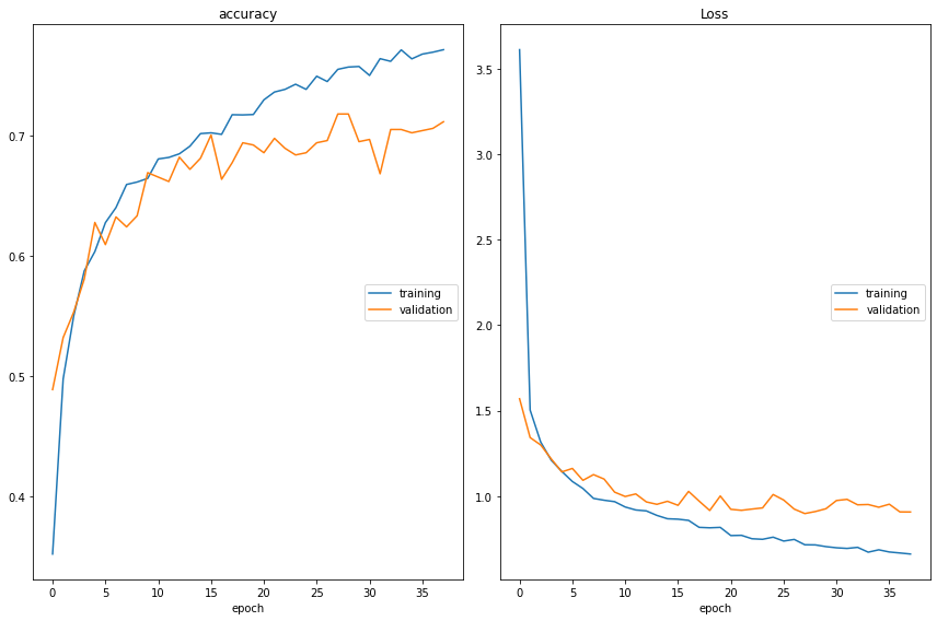
An accuracy of 81%! Amazing what unfreezing the last convolutional layers can do for model performance. Let's get a better idea of how our different models have performed in classifying the data.

Improvements

Recall that our Custom CNN accuracies, Transfer Learning Model with Feature Extraction, and Fine-Tuned Transfer Learning Model are 58%, 73%, and 81%, respectively.

We could see improved performance on our dataset as we introduce fine-tuning. Selecting the appropriate number of layers to unfreeze can require careful experimentation.

Other parameters to consider when training your network include:

• Optimizers: in this article, we used the Adam optimizer to update our weights during training. When training your network, you should experiment with other optimizers and their learning rate.
• Dropout: recall that Dropout is a form of regularization to prevent overfitting of the network. We introduced a single dropout layer in our Fully-Connected layer to constrain the network from over-learning certain features.
• Fully-Connected Layer: if you are taking a bootstrapped approach to Transfer Learning, ensure that your Fully-Connected layer is structured appropriately for the classification task. Is the number of input nodes correct for the outputted features? Do we have too many densely-connected layers?

Summary

In this article, we solved an image classification problem using a custom dataset using Transfer Learning. We saw that by employing various Transfer Learning strategies such as Fine-Tuning, we can generate a model that outperforms a custom-written CNN. Some key takeaways:

1. Transfer learning can be a great starting point for training a model when you do not possess a large amount of data.
2. Transfer learning requires that a model has been pre-trained on a robust source task which can be easily adapted to solve a smaller target task.
3. Transfer learning is easily accessible through the Keras API. You can find available pre-trained models here.
4. Fine-Tuning a portion of pre-trained layers can boost model performance significantly.

          Image classification using vgg16: GitHub link

O